

Introduction
In the era of data-driven decision-making, Linear Regression stands as one of the simplest yet most powerful tools in a data scientist’s arsenal. Whether you’re predicting housing prices, forecasting sales, or analyzing the relationship between variables, Linear Regression provides a straightforward way to derive insights and make predictions based on data.
At its core, Linear Regression is about finding the best-fit line that explains the relationship between an independent variable (input) and a dependent variable (output). Despite its simplicity, the algorithm is a cornerstone of machine learning and statistics, forming the foundation for more complex models like Logistic Regression, Ridge Regression, and Neural Networks.
This article is designed to take you through a practical implementation of Linear Regression using Python. We’ll break down the concept step-by-step, from understanding the underlying theory to evaluating the model’s performance with real data. By the end of this guide, you’ll have a solid understanding of how Linear Regression works and how to apply it to solve predictive modeling problems.
Whether you’re a beginner in machine learning or someone looking to strengthen your fundamentals, this guide will serve as a helpful resource to enhance your understanding of Linear Regression. Let’s dive in!
What is Linear Regression?
Linear regression is a statistical method used to model the relationship between one or more independent variables (X) and a dependent variable (Y). It is widely used in predictive modeling, trend analysis, and inferential statistics.
1. Intuitive Understanding of Linear Regression
Imagine you own a coffee shop, and you want to predict your daily sales (Y) based on the temperature (X).
• You observe that when it’s hotter, more people buy cold drinks, leading to higher sales.
• When it’s colder, sales decrease.
• You plot temperature vs. sales and notice a pattern forming a straight line.
• This means a linear relationship exists between temperature and sales.
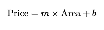
By applying linear regression, you can create a mathematical equation that predicts sales based on temperature:
Y = mX + b
where:
• Y = daily sales (dependent variable)
• X = temperature (independent variable)
• m = slope (how much sales increase per degree of temperature rise)
• b = intercept (sales when the temperature is 0°C)
This equation helps you predict future sales based on temperature trends.
2. Mathematical Derivation of Linear Regression
In statistics, the goal of linear regression is to find the best-fit line that minimizes errors. The most commonly used method to achieve this is the Ordinary Least Squares (OLS) method.
Equation of a Simple Linear Regression Model
Y
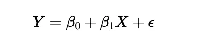
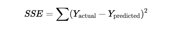
The goal is to minimize the sum of squared errors (SSE):
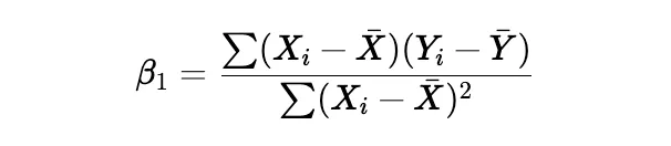
Beta 1:
Beta 0:
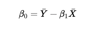
where bar{X} and bar{Y} are the means of X and Y .
These equations determine the best-fit line that minimizes prediction errors.
3. Types of Linear Regression
- Simple Linear Regression
• Involves one independent variable.
• Example: Predicting house prices based on area (sq ft).
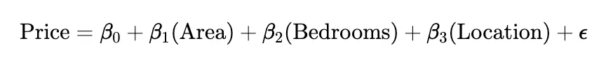
- Multiple Linear Regression
• Involves two or more independent variables.
• Example: Predicting house prices based on area, number of bedrooms, and location.
- Polynomial Regression
• Extends linear regression by adding polynomial terms to capture non-linear relationships.
• Example: Predicting car prices based on age (X²).

- Ridge & Lasso Regression (Regularized Linear Regression)
• Used when there are many independent variables to prevent overfitting.
• Ridge Regression adds a penalty to large coefficients (L2 regularization).
• Lasso Regression selects only the most important variables (L1 regularization).
4. Assumptions of Linear Regression
For linear regression to work well, these assumptions must hold:
- Linearity: The relationship between X and Y is linear.
- Independence: Observations must be independent of each other.
- Homoscedasticity: The variance of residuals (errors) should be constant.
- Normality: Residuals should be normally distributed.
- No Multicollinearity: Independent variables should not be highly correlated.
When these assumptions are violated, linear regression might give biased results.
5. Real-World Applications of Linear Regression
- Finance: Predicting stock prices based on historical trends.
- Healthcare: Estimating patient recovery time based on age and medical history.
- Marketing: Predicting sales based on ad spending.
- Real Estate: Estimating house prices based on square footage and location.
- Manufacturing: Forecasting production costs based on raw material prices.
6. Limitations of Linear Regression
- Assumes Linearity: Doesn’t work well for complex non-linear relationships.
- Sensitive to Outliers: A single extreme data point can distort the model.
- Collinearity Issues: If independent variables are highly correlated, model accuracy decreases.
- Not Always Interpretable: Multiple linear regression models can become complex.
For better accuracy, alternative models like Decision Trees, Random Forests, or Neural Networks are often preferred in real-world scenarios.
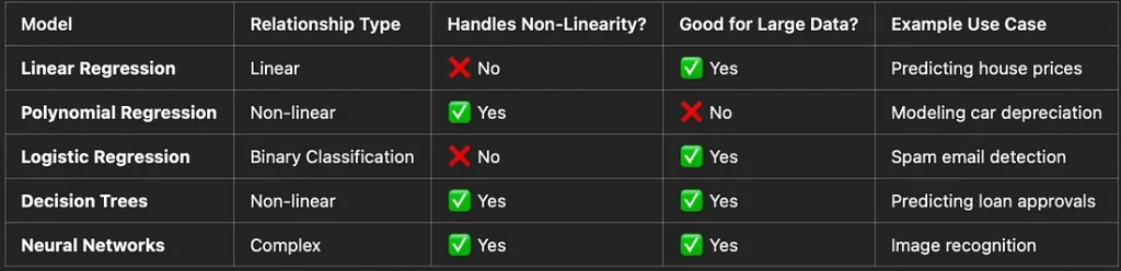
7. Comparing Linear Regression with Other Models
Conclusion
Linear regression is one of the most fundamental machine learning algorithms, used for predicting numerical values. It is easy to interpret, computationally efficient, and works well when relationships are linear. However, it has limitations, especially when data is complex and non-linear. Understanding its assumptions, mathematical foundation, and applications can help you determine when and how to use it effectively.
- Importing Libraries
import numpy as np
import matplotlib.pyplot as plt
• numpy is used for numerical operations, such as creating arrays and performing mathematical calculations.
- matplotlib.pyplot is for plotting graphs (though it’s not utilized directly in this part of the code).
2. Loading the Dataset
df = np.loadtxt("/content/FuelConsumptionCo2.csv", delimiter=",", dtype=str)
display(df)
• The np.loadtxt() function loads data from a CSV file, FuelConsumptionCo2.csv, with comma-separated values. The dataset is read as strings (dtype=str).
- The display(df) shows the dataset, but the display() function is not a standard Python function — it’s likely used for IPython environments like Jupyter notebooks.
3. Extracting Specific Columns
enginesize = df[1:, 4].astype('float64')
fc_comb = df[1:, 10].astype('float64')
co2 = df[1:, 12].astype('float64')
• These lines extract specific columns from the dataset:
• enginesize: Column 4 (index 4) corresponds to engine size.
• fc_comb: Column 10 (index 10) corresponds to fuel consumption.
• co2: Column 12 (index 12) corresponds to CO₂ emissions.
• df[1:, :]: This skips the first row (headers) and selects all rows starting from the second one.
- .astype(‘float64’): Converts the extracted data to numeric type for mathematical operations.
4. Defining the Linear Regression Class
class LinearRegression:
    weights = []
    intercept = 0

    def __init__(self):
        self.weights = []
        self.intercept = 0
• A custom LinearRegression class is defined with two key attributes:
• weights: A list that will store the coefficients for each feature (in this case, engine size and fuel consumption).
- intercept: The y-intercept of the linear regression line.
5. The fit() Method
def fit(self, X, y):
    y = y.astype('float64')
    ms = []
    for x in X:
        x = x.astype('float64')
        a = sum((x - np.mean(x)) * (y - np.mean(y))) / sum((x - np.mean(x)) ** 2)
        self.weights.append(a)
        ms.append(a * np.mean(x))
    b = np.mean(y) - sum(ms)
    self.intercept = b
• The fit() method is responsible for training the model. It computes the weights (coefficients) for the features and the intercept using the formula for Linear Regression.
- First, it calculates the slope (weight) using the formula:
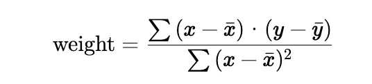
This is equivalent to the covariance between x and y divided by the variance of x .
• The intercept b is calculated as:
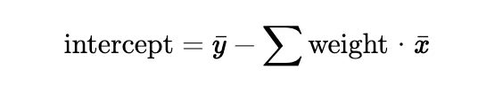
- The calculated weights and intercept are stored in the class attributes (weights and intercept).
6. The predict() Method
def predict(self, X):
    ms = []
    for i in range(len(self.weights)):
        x = X[i].astype('float64')
        ms.append(self.weights[i] * np.mean(x))
    y = sum(ms) + self.intercept
    print(y)
• The predict() method makes predictions based on the fitted model:
• It computes the predicted values by multiplying the weights with the features and summing them up.
• The intercept is added to the final prediction.
- The result is printed.
7. Fitting the Model and Making Predictions
l1 = LinearRegression()
l1.fit(np.array([enginesize, fc_comb]), co2)
l1.predict(np.array([enginesize, fc_comb]))
• An instance of the LinearRegression class (l1) is created.
• The fit() method is called with engine size (enginesize) and fuel consumption (fc_comb) as input features and CO₂ emissions (co2) as the target variable.
- The predict() method is then called to make predictions based on the fitted model.
Key Points to Note:
• Multiple Features: The code is using two features (enginesize and fc_comb) to predict CO₂ emissions. However, the current implementation treats them independently by iterating over each feature separately, which may not be the ideal approach for multiple linear regression.
• Simple Linear Regression Approach: The custom implementation follows a basic linear regression approach. While this approach works, libraries like scikit-learn offer optimized methods for fitting and predicting models.
- Prediction: The predict() method here adds the predicted values together, but this approach might be mathematically incorrect because it should consider each feature’s contribution independently (weighted by the coefficients for each feature).
Suggestions for Improvement:
• Vectorized Computation: Instead of iterating through each feature and calculating the mean, you could use vectorized operations for efficiency.
- Proper Multiple Linear Regression: In a true multiple linear regression, you’d multiply each feature by its respective coefficient and sum them up rather than adding the predictions from each feature independently.
Conclusion
Linear Regression is a powerful and foundational technique in statistics and machine learning, used to model the relationship between a dependent variable and one or more independent variables. Through the process of fitting a linear model, we determine the best-fitting line (or hyperplane in higher dimensions) that minimizes the difference between the predicted and actual values.
In this article, we explored how linear regression works and how to implement it from scratch using Python. We used simple mathematical formulas to compute the weights and intercept, and learned how these parameters influence the model’s predictions.
By understanding and implementing linear regression, we gain valuable insights into the underlying patterns of the data, which can be applied to a wide variety of fields, including economics, biology, engineering, and more. Although advanced libraries like scikit-learn provide optimized solutions, building the model from the ground up allows us to deepen our understanding of the underlying mathematical principles.
In summary, linear regression remains an essential tool for anyone working with predictive modeling, providing a clear and interpretable way to make predictions based on existing data.
Full code:
import numpy as np
import matplotlib.pyplot as plt

# using loadtxt()
df = np.loadtxt("/content/FuelConsumptionCo2.csv",
                 delimiter=",", dtype=str)
display(df)


enginesize = df[1:, 4].astype('float64')
print(enginesize)

fc_comb = df[1:, 10].astype('float64')
print(fc_comb)

co2 = df[1:, 12].astype('float64')
print(co2)


class LinearRegression:
    weights = []
    intercept = 0

    def __init__(self):
        self.weights = []
        self.intercept = 0

    def fit(self, X, y):
        y = y.astype('float64')
        ms = []
        for x in X:
            x = x.astype('float64')
            a = sum((x - np.mean(x)) * (y - np.mean(y))) / sum((x - np.mean(x)) ** 2)
            self.weights.append(a)
            ms.append(a * np.mean(x))
        b = np.mean(y) - sum(ms)
        self.intercept = b

    def predict(self, X):
        ms = []
        for i in range(len(self.weights)):
            x = X[i].astype('float64')
            ms.append(self.weights[i] * np.mean(x))
        y = sum(ms) + self.intercept
        print(y)


l1 = LinearRegression()
l1.fit(np.array([enginesize, fc_comb]), co2)
l1.predict(np.array([enginesize, fc_comb]))
Feel free to visit my GitHub profile to explore more of my projects and connect with me!