Gradient Descent: A Comprehensive Guide

What is Gradient Descent?

Gradient descent is an optimization algorithm used to minimize a function by iteratively moving in the direction of the negative gradient. It is widely used in machine learning for optimizing cost functions and finding the best parameters for a model.

In simple terms, gradient descent helps find the lowest point of a function (such as an error function) by taking small steps in the direction that reduces the function’s value the most. Imagine a person walking down a mountain in thick fog — they would move in the steepest downward direction at each step, adjusting their path as the terrain changes.

Why is Gradient Descent Important?

In machine learning, we often deal with large datasets and complex models that require efficient optimization techniques. Gradient descent allows us to train models faster by iteratively improving model parameters and reducing error. It is particularly useful when dealing with functions that have multiple variables and a large number of data points, making it computationally infeasible to find a direct mathematical solution.

Types of Gradient Descent

There are three main types of gradient descent, each with its own advantages and trade-offs:

1. Batch Gradient Descent: Uses the entire dataset to compute the gradient before updating parameters. This ensures stable convergence but can be slow for large datasets.
2. Stochastic Gradient Descent (SGD): Updates parameters using a single randomly selected data point per iteration, making it faster but more noisy.
3. Mini-Batch Gradient Descent: A compromise between batch and stochastic methods, using a small subset (batch) of data points for each update. This balances speed and stability.

How Does Gradient Descent Work?

Gradient descent follows these steps:

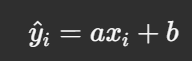
1. Initialize Parameters: Start with initial values for parameters (e.g., a and b).
2. Compute Predictions: Calculate the predicted values (y_hat).
3. Calculate Error (MSE): Compute the Mean Squared Error (MSE) as the cost function.
4. Compute Gradients: Calculate grad_a and grad_b to find the direction of steepest descent.
5. Update Parameters: Adjust a and b using the gradients and a learning rate.
6. Repeat Until Convergence: Continue updating parameters until MSE stops decreasing significantly.

How to Calculate Mean Squared Error (MSE)?

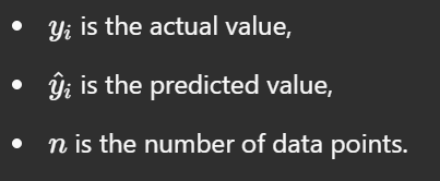
MSE measures the average squared difference between the actual values and the predicted values:

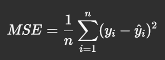
where:

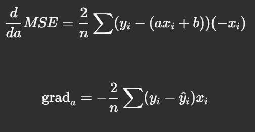
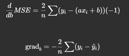
How are grad_a and grad_b Derived?

To minimize MSE using gradient descent, we take partial derivatives of MSE with respect to a and b.

Derivation of grad_a

The predicted values are given by:

Substituting this into the MSE formula:

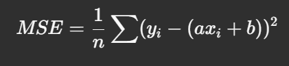
Taking the derivative with respect to a:

Derivation of grad_b

Taking the derivative of MSE with respect to b:

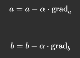
How MSE Changes After Updating a and b

Using the gradients, we update our parameters:

Choosing the Learning Rate

The learning rate determines the step size in gradient descent. A proper learning rate should be neither too small nor too large:

• Small Learning Rate: Leads to slow convergence.
• Large Learning Rate: Can cause overshooting or divergence.

What is Convergence?

Convergence refers to the process where the gradient descent algorithm approaches a point where further iterations do not result in significant changes to the model parameters or the cost function. Here’s a more detailed explanation:

• Gradient Descent Overview: Gradient descent is an optimization algorithm used to minimize the cost function (e.g., Mean Squared Error, MSE) by iteratively adjusting the model parameters (weights) in the direction of the steepest descent (negative gradient).
• Cost Function: The cost function measures how well the model’s predictions align with the actual data. In the case of MSE, it calculates the average squared difference between predicted and actual values.
• Small Updates: As the algorithm progresses, the updates to the parameters become smaller. This is often quantified by a threshold; when the change in the cost function is below this threshold, the algorithm is considered to have converged.
• Optimal Solution: Convergence indicates that the algorithm has likely found an optimal or near-optimal solution where the cost function is minimized. However, it’s important to note that convergence does not always mean the global minimum has been reached, especially in non-convex functions.

What is Overshooting or Divergence?

Overshooting and divergence are issues that can arise during the training process, particularly related to the learning rate:

Overshooting

• Definition: Overshooting occurs when the learning rate is set too high, causing the algorithm to make large jumps in parameter space. Instead of gradually approaching the optimal solution, the updates are so large that they overshoot the minimum.
• Effect: When overshooting occurs, the algorithm may oscillate around the optimal solution without settling down. This can lead to erratic behavior in the cost function, where it fails to stabilize and may even start increasing.

Divergence

• Definition: Divergence is a more severe case than overshooting. It happens when the updates are excessively large, causing the parameters to move away from the optimal solution instead of towards it.
• Effect: When divergence occurs, the cost function does not just fail to decrease; it increases indefinitely. This is typically a sign that the learning rate is too high or that there are issues with the data or model configuration.

Convergence is the desired outcome of gradient descent, indicating that the algorithm has found a stable point where further updates lead to minimal changes in the cost function.

Overshooting and divergence are problems that can arise from a learning rate that is too high, leading to instability and failure to minimize the cost function effectively.

Recommendations

• Learning Rate Tuning: It’s essential to carefully tune the learning rate. Techniques like learning rate schedules or adaptive learning rates (e.g., Adam optimizer) can help mitigate these issues.
• Monitoring: Always monitor the cost function during training to identify convergence, overshooting, or divergence early on, allowing for adjustments as needed.

Example Calculation

Given:

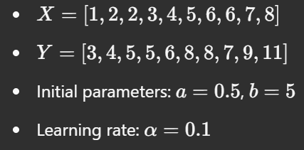
Step 1: Compute Predictions

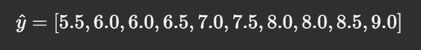
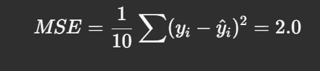
Step 2: Compute MSE

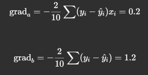
Step 3: Compute Gradients

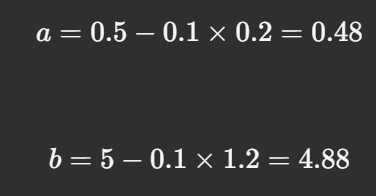
Step 4: Update Parameters

Step 5: Recalculate MSE

After updating:

This process continues iteratively until MSE converges to a minimal value, achieving the best-fit line for our data.

This extended guide provides a more in-depth discussion of gradient descent, including its importance, derivations, and practical applications. Let me know if you’d like further refinements or additional examples!