

Introduction
Regression analysis is one of the foundational techniques in machine learning and data science. It helps us understand relationships between variables and make predictions about future outcomes. However, building a regression model is only half the journey — the true challenge lies in evaluating its performance. This is where loss functions and accuracy metrics come into play.
Loss functions measure how well a model’s predictions align with actual outcomes, while accuracy metrics provide a quantifiable assessment of a model’s performance. By understanding these concepts, data practitioners can not only assess their models effectively but also identify areas for improvement.
In this article, we’ll explore key loss functions used in regression, including Mean Absolute Error (MAE) and Mean Squared Error (MSE). Additionally, we’ll discuss the R² score, a metric that indicates how well the model explains the variability in the target data. Through hands-on examples, we’ll demonstrate how these metrics work and why they matter.
Whether you’re a beginner stepping into the world of machine learning or someone looking to refine their understanding of regression metrics, this guide will serve as a valuable resource. Let’s dive in!
1. What Are Loss Functions and Why Do They Matter?
Loss functions are mathematical functions that measure the difference between predicted and actual values. In regression, loss functions help assess how well the model is performing by quantifying the errors. By minimizing the loss, we can optimize the model to make better predictions.
• Role in optimizing regression models: Loss functions guide the training of regression models. The model aims to minimize the loss, which means it’s adjusting its parameters to reduce the discrepancy between predicted and actual values.
• Examples:
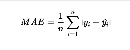
• Mean Absolute Error (MAE): Measures the average magnitude of errors in predictions, without considering their direction.
• Mean Squared Error (MSE): Measures the average of the squared differences between actual and predicted values, emphasizing larger errors.
2. Key Loss Functions in Regression
• Mean Absolute Error (MAE):
• Explanation: MAE calculates the average of the absolute differences between predicted and actual values.
• Formula:
• Pros: Easy to understand and less sensitive to outliers.
• Cons: Doesn’t penalize larger errors as much as MSE.
• Mean Squared Error (MSE):
• Explanation: MSE calculates the average of the squared differences between actual and predicted values.
• Formula:
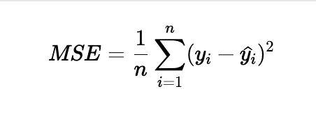
• Why MSE penalizes larger errors: Since MSE squares the errors, larger errors are given more weight, which can help in situations where large deviations need to be minimized.
• Comparison of MAE and MSE:
• Example: Use a simple dataset to show how MAE and MSE evaluate the errors differently, especially when there are large discrepancies.
3. Understanding R² Score
• Explanation: The R² score, or coefficient of determination, is a measure of how well the regression model fits the data.
• Formula:
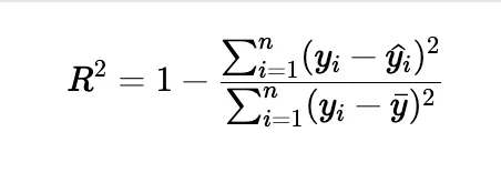
• Interpreting R²: A higher R² score (closer to 1) indicates a better fit, while a lower R² score suggests the model doesn’t explain much of the variance in the data.
4. Hands-On Example: Implementing Linear Regression
• Walk through the code for implementing a basic linear regression model.
• Show how to calculate MAE, MSE, and R² as part of the evaluation process.
5. Why Evaluating Regression Models Is Crucial
• Balancing underfitting and overfitting: Emphasize how evaluating models with loss functions and accuracy metrics helps find the right balance.
• Choosing the right loss function: Discuss how the choice of loss function depends on the dataset and the goal (e.g., handling outliers, prioritizing larger errors).
• Improving models: Highlight how iterating based on evaluation metrics can lead to better models.
6. Conclusion
• Recap the key points about loss functions and accuracy metrics.
• Encourage readers to experiment with different loss functions and accuracy measures.
• Invite feedback and questions to foster engagement.
Hands-On Example: Implementing Linear Regression
In this section, I will explain the code for implementing a simple linear regression model, which is the most basic model for predicting a dependent variable based on an independent variable. We will also calculate three key evaluation metrics — Mean Absolute Error (MAE), Mean Squared Error (MSE), and R² Score — to assess how well our model performs.
Code Walkthrough:
- Defining the Data:
x_data = np.array([2, 2.5, 2.5, 3, 3.2, 3.5, 4, 4, 4, 4.5, 4.7, 4.8, 5, 5, 5.5])
y_data = np.array([5, 5, 6.5, 6, 7, 7.5, 7.5, 7, 8.5, 8, 8, 8.5, 10, 10.5, 11])
Here, x_data represents the independent variable (input), and y_data represents the dependent variable (target values). We use a small dataset for demonstration purposes.
2. Creating the Linear Regression Class:
class LinearRegression:
    weights = []
    intercept = 0

    def __init__(self):
        self.weight = 0
        self.intercept = 0
We define a custom LinearRegression class with a constructor (__init__) to initialize the weight and intercept of the model. These values are crucial for predicting new data points.
3. Fitting the Model:
def fit(self, x, y):
    x_bar = np.float64(format(np.mean(x), ".2f"))
    y_bar = np.float64(format(np.mean(y), ".2f"))
    a = np.float64(format(sum(((x - x_bar) * (y - y_bar))) / sum(((x - x_bar) ** 2)), ".2f"))
    b = np.float64(format(y_bar - (a * x_bar), ".2f"))
    self.weight = a
    self.intercept = b
    return
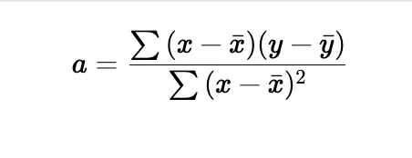
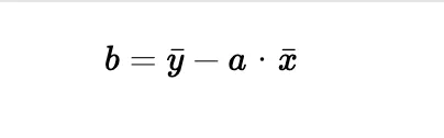
In the fit() method, we calculate the slope (a) and the intercept (b) for the linear regression line using the formula for the least squares method:
In the fit() method, we calculate the slope (a) and the intercept (b) for the linear regression line using the formula for the least squares method:
• Slope (a):
• Intercept (b):
After calculating the values for a and b, we store them in the class’s instance variables weight and intercept.
4. Making Predictions:
def predict(self, x):
    predicts = (self.weight * x + self.intercept)
    predicts = np.array(list(map(lambda s: np.float64(format(s, ".2f")), predicts)))
    return predicts
In the predict() method, we use the formula for a linear regression model:

We apply this formula to each value of x in the dataset and round the predictions to two decimal places for consistency.
5. Initializing the Model and Fitting the Data:
l1 = LinearRegression()
l1.fit(x_data, y_data)
y_hats = l1.predict(x_data)
We create an instance of the LinearRegression class, fit the model using the provided x_data and y_data, and make predictions (y_hats) for the input data.
6. Calculating MAE, MSE, and R²:
mae = np.float64(format(sum(abs(y_data - y_hats)) /len(y_data), ".2f"))
mse = np.float64(format(sum(((y_data - y_hats) ** 2)) / len(y_data), ".2f"))
y_bar = np.float64(format(np.mean(y_data), ".2f"))
r2_score = np.float64(format(1 - (sum(((y_data - y_hats) ** 2))) / sum(((y_data - y_bar) ** 2)), ".2f"))
• MAE: The Mean Absolute Error measures the average of the absolute differences between predicted and actual values. It gives us an indication of how far off our predictions are on average.
• MSE: The Mean Squared Error penalizes larger errors more than smaller ones by squaring the difference. It provides a way to emphasize larger deviations.
• R²: The R² score, also called the coefficient of determination, indicates how well the model explains the variance of the data. A higher R² value means a better fit.
Each metric is calculated using numpy functions, and we round the results to two decimal places for consistency.
7. Displaying Results:
print(mae)
print(mse)
print(r2_score)
Finally, we print the values of MAE, MSE, and R² for the model’s evaluation. These metrics will give us a clear idea of how well our linear regression model has performed on the given dataset.
import numpy as np

x_data = np.array([2, 2.5, 2.5, 3, 3.2, 3.5, 4, 4, 4, 4.5, 4.7, 4.8, 5, 5, 5.5])
y_data = np.array([5, 5, 6.5, 6, 7, 7.5, 7.5, 7, 8.5, 8, 8, 8.5, 10, 10.5, 11])

class LinearRegression:
    weights = []
    intercept = 0

    def __init__(self):
        self.weight = 0
        self.intercept = 0

    def fit(self, x, y):
        x_bar = np.float64(format(np.mean(x), ".2f"))
        y_bar = np.float64(format(np.mean(y), ".2f"))
        a = np.float64(format(sum(((x - x_bar) * (y - y_bar))) / sum(((x - x_bar) ** 2)), ".2f"))
        b = np.float64(format(y_bar - (a * x_bar), ".2f"))
        self.weight = a
        self.intercept = b
        return

    def predict(self, x):
        predicts = (self.weight * x + self.intercept)
        predicts = np.array(list(map(lambda s: np.float64(format(s, ".2f")), predicts)))
        return predicts

l1 = LinearRegression()
l1.fit(x_data, y_data)
y_hats = l1.predict(x_data)

mae = np.float64(format(sum(abs(y_data - y_hats)) /len(y_data), ".2f"))
mse = np.float64(format(sum(((y_data - y_hats) ** 2)) / len(y_data), ".2f"))
y_bar = np.float64(format(np.mean(y_data), ".2f"))
r2_score = np.float64(format(1 - (sum(((y_data - y_hats) ** 2))) / sum(((y_data - y_bar) ** 2)), ".2f"))

print(mae)
print(mse)
print(r2_score)
Conclusion
In this example, we demonstrated how to implement a basic linear regression model from scratch and calculate important evaluation metrics such as MAE, MSE, and R². These metrics are crucial for understanding the performance of a model and guiding future improvements.
Feel free to visit my GitHub profile to explore more of my projects and connect with me!